Approximate Nearest Neighbor Search and HNSW
On this page
Learning Objective
Explain conceptually how HNSW navigates a layered proximity graph to find near neighbors without scanning the corpus, describe what the M, ef_construction, and ef_search parameters actually control, and compare HNSW with IVF and quantization-based indexes on memory, build cost, and update behavior.
Concept Explanation
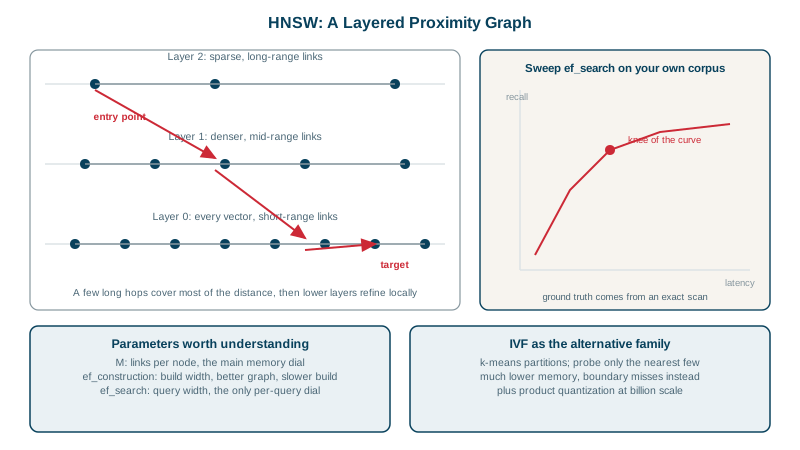
Hierarchical Navigable Small World, introduced by Malkov and Yashunin, is the dominant approximate nearest neighbor index in current systems, and the intuition behind it is more approachable than the name suggests. Build a graph where each vector is a node connected to some of its nearest neighbors. To search, start anywhere, look at the current node's neighbors, move to whichever is closer to the query, and repeat until no neighbor is closer. This is greedy descent through a proximity graph, and it works because a graph of nearest-neighbor links is navigable: local moves make consistent progress toward any target. The problem with a single flat graph is that if you start far away, reaching the target takes a long walk of many small steps.
The hierarchy fixes exactly that. HNSW builds multiple layers, assigning each node a maximum layer drawn from an exponentially decaying distribution, so the top layer contains very few nodes with long-range connections and each layer down contains more nodes with progressively shorter-range connections, with the bottom layer containing everything. Search starts at the single entry point in the sparse top layer and greedily descends, and because the top layers have long-range links, the first few hops cover enormous distance and land the search in approximately the right region. Lower layers then refine locally. It is the same structural idea as a skip list applied to a proximity graph instead of a sorted list, and it turns a long linear walk into a logarithmic descent.
Three parameters govern the tradeoff and they are worth understanding rather than copying from a tutorial. M is the maximum number of bidirectional links per node per layer, and it is the primary memory dial: memory grows roughly linearly in M, while higher M gives better recall especially on high-dimensional or clustered data. Typical values sit between 12 and 64. The parameter ef_construction controls how large a candidate list is explored when inserting each node during the build, so higher values produce a better-connected, higher-recall graph at the cost of longer build time, with no runtime memory cost. The parameter ef_search is the query-time equivalent: it sets the size of the dynamic candidate list during search, and it is the one knob tunable per query without rebuilding, trading latency directly for recall. It must always be at least k, and raising it is the first thing to try when recall is too low.
The main alternative family is inverted file indexes, IVF. Rather than a graph, the vectors are clustered by k-means into a number of partitions, each with a centroid. A query compares against the centroids, selects the few nearest partitions, and scans only those. This makes the memory overhead minimal compared to HNSW, since you store centroids plus assignments rather than a dense link structure, and it makes the build a clustering pass rather than an incremental graph construction. Its weakness is boundary effects: a true neighbor sitting just across a partition boundary is missed unless you probe more partitions, and the training step means the index reflects the data distribution at build time, so a corpus that drifts substantially needs retraining. IVF is commonly combined with product quantization, which compresses each vector into a short code by splitting it into subvectors and replacing each with the nearest entry from a learned codebook, cutting memory by an order of magnitude or more at a real cost in precision that is typically recovered by rescoring the top candidates against full-precision vectors.
Two operational realities matter more in production than the theory. First, updates. HNSW supports incremental inserts naturally, but deletes are typically soft, marking a node as removed while leaving it in the graph for navigation, which means a corpus with heavy churn accumulates tombstones and degrades until a rebuild or compaction. IVF handles bulk rebuilds well but incremental inserts drift away from centroids trained on older data. Second, the parameters interact with your actual data distribution, so recall measured on a public benchmark is not your recall. The only trustworthy procedure is to take a sample of your real corpus, compute exact nearest neighbors by brute force as ground truth, and sweep ef_search to find the recall-versus-latency point your product actually needs, which is frequently lower than the default and therefore cheaper.
| Index | Memory | Build Cost | Query Speed | Updates | Best Fit |
|---|---|---|---|---|---|
| Flat (exact) | Vectors only | None | Linear in corpus size | Trivial | Under a few hundred thousand vectors |
| HNSW | High: vectors plus a dense link graph | Slow incremental build | Fastest at high recall | Inserts fine; deletes are soft and accumulate | Latency-critical search that fits in RAM |
| IVF | Low: centroids plus assignments | A k-means training pass | Good, tuned by how many partitions are probed | Inserts drift from trained centroids | Large corpora where memory is the constraint |
| IVF plus product quantization | Very low: compressed codes | Training plus codebook learning | Very fast, lower precision | Same drift as IVF | Billion-scale corpora with rescoring on top |
Worked Example: Tuning ef_search Against Measured Ground Truth
The procedure below is the only honest way to pick these parameters. Exact search on a sample gives ground truth, and the sweep tells you where your own recall-latency curve bends, which is usually well before the default value anyone recommends.
-- Build once, with the memory and build-time dials.
CREATE INDEX chunks_hnsw ON chunks
  USING hnsw (embedding vector_cosine_ops)
  WITH (m = 16, ef_construction = 128);
--   m = 16            -> link budget per node; the main MEMORY dial
--   ef_construction   -> build-time search width; better graph, slower build,
--                        costs nothing at query time

-- Tune per query, without rebuilding anything.
SET hnsw.ef_search = 40;   -- must be >= k; the main RECALL/LATENCY dial

/*  Measurement procedure - do not skip the ground truth step.

 1. Sample 1,000 real queries from production logs (not synthetic ones:
    the query distribution determines where in the space you land).
 2. Compute the TRUE top-10 for each by exact brute force over the corpus
    sample. This is the only ground truth that exists.
 3. Sweep ef_search and measure both numbers together:

      ef_search   recall@10   p95 latency
         10         0.78         3 ms
         40         0.94         7 ms     <- knee of the curve
         100        0.98        16 ms
         400        0.995       58 ms     <- 5.5% recall for 8x the latency

 4. Pick against the PRODUCT requirement. A re-ranking stage downstream
    (Lesson 9) makes low-90s recall perfectly adequate, because the
    re-ranker fixes ordering - it just cannot recover what was never
    retrieved. Paying 58 ms for 0.995 here is usually wasted budget.
*/
Real-World Examples
- The HNSW algorithm was published by Yury Malkov and Dmitry Yashunin, appearing on arXiv in 2016 and in IEEE Transactions on Pattern Analysis and Machine Intelligence in 2018, and it has since become the default approximate nearest neighbor index in a remarkably wide set of systems including Lucene, pgvector, Qdrant, Weaviate, and Milvus, which is an unusual degree of convergence on a single data structure.
- The public ann-benchmarks project maintains reproducible comparisons of approximate nearest neighbor implementations across standard datasets, plotting recall against queries per second, and it consistently shows that no implementation dominates across all datasets and recall targets. That is the empirical basis for the rule that index parameters must be tuned against your own corpus and query distribution rather than copied from someone else's benchmark.
Review Questions & Answers
A single flat proximity graph only has short-range links, so reaching a distant target requires many small hops and the walk length grows with the size of the corpus. HNSW assigns nodes to layers from an exponentially decaying distribution, so the top layers are sparse and their links span long distances. The search starts at the top and covers most of the distance to the target region in a handful of very long hops, then descends into progressively denser layers that refine the result locally. It is the same mechanism a skip list uses to turn a linear list traversal into a logarithmic one, applied to a proximity graph instead of a sorted sequence.
ef_construction controls how widely the algorithm searches for good neighbors when inserting each node during the build, so it determines the quality of the graph's connectivity. It costs build time but nothing at query time, and changing it requires rebuilding the index. ef_search controls the size of the dynamic candidate list during a query, so it trades query latency for recall directly and can be changed per query with no rebuild. Raise ef_search first, because it is free to try, immediately measurable, and reversible. Only if the recall-latency curve is unacceptable at every ef_search value does the graph itself need rebuilding with a higher M or ef_construction.
IVF partitions the space into clusters and scans only the partitions whose centroids are nearest the query, so a true nearest neighbor that happens to sit just on the other side of a partition boundary is never examined unless more partitions are probed. The miss is caused by a hard geometric partition of the space. HNSW has no partitions; its misses come from greedy descent settling in a local region and not exploring widely enough, which is why widening the candidate list at query time directly reduces them. IVF additionally has a distribution-drift problem HNSW does not, because its centroids are trained on the corpus as it existed at build time.
Because the two stages fix different problems. The approximate index determines which candidates exist at all, and the re-ranker determines their order. A re-ranker can promote a correct chunk that the index returned in position forty to position one, but it can do nothing about a chunk the index never returned. What matters, therefore, is whether the correct chunk is in the candidate set, not whether the index ranked it perfectly. Since candidate sets are typically fifty or more items while the recall figure is usually quoted at ten, the effective recall at the size that matters is considerably higher, which means paying several times the latency to move a quoted recall figure from 0.94 to 0.995 usually buys no end-to-end improvement at all.