Sharding Strategies: Range vs Hash vs Directory
On this page
Learning Objective
Distinguish vertical from horizontal partitioning, compare range, hash, and directory-based sharding on distribution, range-query support, and rebalancing cost, and explain why the choice determines which queries will be cheap for the lifetime of the system.
Concept Explanation
Sharding means splitting one logical dataset across multiple independent database instances so that no single machine holds all of it. It is worth being precise about what problem this solves, because it is frequently reached for when something cheaper would do. Sharding addresses write throughput exceeding one primary, dataset size exceeding one machine storage or memory, and, in some designs, blast radius isolation. It does not address read throughput, which read replicas handle with vastly less complexity, and it is not a general performance technique. Because sharding makes cross-shard operations expensive and permanently complicates the data layer, the correct order of operations is to exhaust indexing, query optimization, caching, read replicas, and vertical scaling first, and to shard when a specific, measured limit has actually been reached.
Vertical partitioning splits by column or by table: move the rarely-read large text blob into its own table or service, or separate the orders tables from the analytics tables onto different machines. It is genuinely useful, it is often the right first step, and it is bounded, because eventually one of the resulting pieces is itself too large for one machine. Horizontal partitioning splits by row: every shard has the same schema and holds a disjoint subset of the rows, chosen by a shard key. That is unbounded in principle, which is why it is the technique that matters at scale, and it comes in three main flavours distinguished by how a row is mapped to a shard.
Range-based sharding assigns contiguous ranges of the shard key to shards: customer ids 1 to 1,000,000 on shard 1, and so on, or, very commonly, time ranges with each month on its own shard. Its enormous advantage is that range queries and ordered scans are efficient, because the rows a query wants are contiguous and usually live on one shard. Its equally enormous disadvantage is that real key distributions are not uniform, and sequential keys are pathological: with an auto-incrementing id or a timestamp as the shard key, every single insert goes to the highest range, so one shard absorbs the entire write load while the others are idle. This is the single most common sharding mistake and it produces a system with all the complexity of sharding and none of the write scaling.
Hash-based sharding applies a hash function to the shard key and maps the result to a shard, usually through consistent hashing or through a fixed number of virtual buckets. The distribution is excellent essentially by construction, because a good hash destroys whatever skew existed in the input, and sequential keys are no longer a problem at all. What it destroys along with the skew is ordering: adjacent keys land on unrelated shards, so any range query must be broadcast to every shard and the results merged, which converts a cheap operation into a scatter-gather across the fleet. Hash sharding also makes it awkward to migrate a specific tenant or to co-locate related rows unless the key is chosen carefully, which is why most real hash-sharded systems use a compound key whose prefix groups related rows.
Directory-based sharding introduces an explicit lookup service or table that maps a key, or a group of keys, to a shard. It is the most flexible option by a wide margin: any key can be moved to any shard at any time by updating one entry, a large tenant can be given a dedicated shard, and the mapping can encode arbitrary business rules such as data residency. The costs are that every operation needs the mapping, so it must be cached aggressively and kept highly available, and the directory becomes a critical dependency whose failure takes down all data access. In practice most large systems converge on a hybrid: a fixed, generous number of logical shards assigned by hashing, plus a directory mapping logical shards to physical instances. Hashing gives the even distribution, and the indirection layer gives the ability to move logical shards between physical machines without ever changing how a key maps to a logical shard. This is the structure behind several well-known production designs and it is worth adopting from the start, because retrofitting the indirection later is far harder than including it.
| Strategy | Distribution | Range Queries | Rebalancing | Typical Failure |
|---|---|---|---|---|
| Range-based | Poor with real-world or sequential keys | Efficient; contiguous rows on one shard | Split a hot range, which is straightforward | All writes land on the newest range |
| Hash-based | Excellent by construction | Requires scatter-gather across every shard | Needs consistent hashing or a fixed bucket count | Range and ordered queries become fleet-wide |
| Directory-based | Fully controllable, including per-tenant | Depends on how the directory groups keys | Easiest; update one mapping entry | The directory is a critical dependency and a bottleneck |
| Hash into logical shards, directory to physical | Excellent | Scatter-gather, unless the key prefix groups rows | Move a logical shard without remapping any key | Requires planning the logical shard count up front |
Worked Example: Logical Shards Behind a Physical Map
The pattern below is what large systems converge on, and the reason is in the last few lines: growing the fleet never changes which logical shard a key belongs to, so no key ever moves between logical shards and only whole logical shards move between machines.
# Choose a fixed, generous logical shard count ONCE, at design time.
# It must be far larger than any plausible physical machine count and
# should be a power of two so the modulo is a mask.
LOGICAL_SHARDS = 4096

def logical_shard(shard_key):
    return crc32(str(shard_key)) % LOGICAL_SHARDS     # never changes, ever

# The physical map is small, cached everywhere, and is the only thing
# that changes when the fleet grows.
physical_map = {
    range(0,    1024): "db-01",
    range(1024, 2048): "db-02",
    range(2048, 3072): "db-03",
    range(3072, 4096): "db-04",
}

def route(shard_key):
    ls = logical_shard(shard_key)
    return physical_map.lookup(ls)

# --- Growing from 4 machines to 8 ---
# Each existing machine hands 512 of its 1024 logical shards to a new one.
# What moves:  whole logical shards (a bulk copy, then a cutover).
# What does NOT move: the key -> logical shard mapping. Not one key
# changes its logical shard, so application code, caches keyed by shard,
# and any denormalized references remain valid throughout.
#
# Contrast with hashing straight to machines:  crc32(key) % 4 -> % 8
# remaps roughly half of ALL keys, requiring a full data reshuffle.

# --- Compound keys keep related rows together ---
# Bad:  shard on message_id       -> one conversation's messages scatter
#                                    across every shard; reading a thread
#                                    is a 4096-way scatter-gather.
# Good: shard on conversation_id  -> the whole thread lives on one shard;
#                                    reading it is a single-shard query.
logical_shard(conversation_id)     # rows: (conversation_id, message_id, ...)

# --- The sequential-key trap, stated plainly ---
# Range sharding on an auto-increment id or a timestamp:
#   shard 1: ids       1 - 1,000,000   0 writes/sec   (all historical)
#   shard 2: ids 1,000,001 - 2,000,000  0 writes/sec
#   shard 3: ids 2,000,001 - 3,000,000  0 writes/sec
#   shard 4: ids 3,000,001 -    ...     ALL writes/sec  <-- the only one
# You now operate four databases and have the write capacity of one.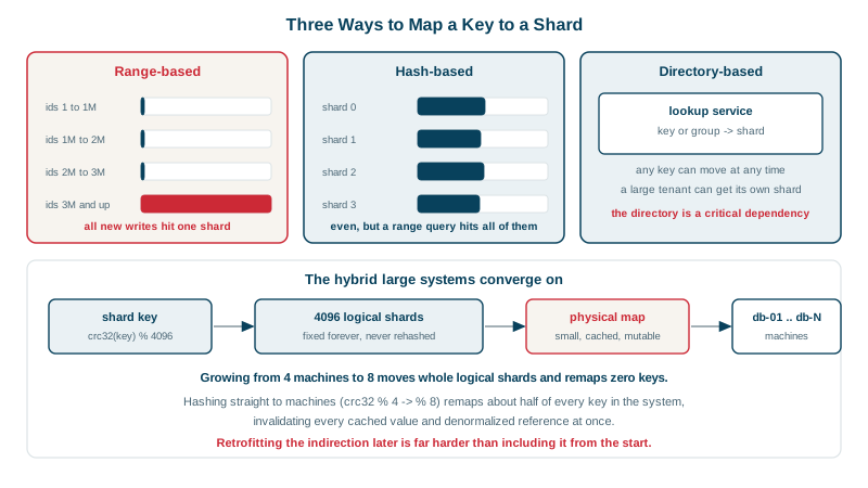
Real-World Examples
- Instagram published its early sharding design in 2012, describing thousands of logical shards implemented as PostgreSQL schemas distributed across a much smaller number of physical machines, specifically so that growth meant moving logical shards to new hardware rather than recomputing which shard a row belongs to. Its companion post on ID generation explains that the shard identifier is embedded directly in the 64-bit id, so any object id alone is sufficient to locate its shard without a lookup.
- Pinterest described sharding its MySQL fleet with a fixed set of virtual shards encoded into a 64-bit id alongside the type and local id, chosen up front at a count large enough that they would never need to change it, and mapped to physical hosts through a configuration layer. The published rationale is precisely the one in this lesson: adding capacity should move shards, never rehash keys, because rehashing keys invalidates every denormalized reference and cached value in the system at once.
Review Questions & Answers
Sharding splits data so each shard holds a subset, which divides write load and storage but does nothing inherent for reads, since a read for a given row still goes to exactly one machine and that machine capacity for serving it is unchanged. Meanwhile sharding imposes permanent costs: cross-shard queries become scatter-gather, transactions across shards require distributed coordination, joins between differently-sharded tables become application-level work, and every future schema change must be applied N times. Read replicas solve read throughput directly by adding machines that each hold a full copy and can serve any read, requiring no change to the data model, no shard key decision, and no query restrictions, at the cost of replication lag. Replicas should therefore be exhausted before sharding is considered, and the two are complementary rather than alternatives once sharding is genuinely required.
Hashing is designed to destroy the relationship between input proximity and output proximity, so two keys that are adjacent in value produce hashes that are unrelated and therefore land on unrelated shards. A query for a contiguous range of keys has no way to know which shards hold members of that range, so it must be sent to every shard, each shard performs a local scan, and the coordinator merges the results. The query cost grows with fleet size rather than with result size, and its latency is governed by the slowest shard. A compound shard key fixes this for the grouping that matters by hashing only a prefix, so all rows sharing that prefix land on the same shard and remain locally ordered by the rest of the key. A messages table keyed on conversation id plus timestamp lets a query for one conversation recent messages be a single-shard ordered scan, while still distributing conversations evenly across the fleet.
It decouples the key-to-shard mapping from the fleet size, so the fleet can grow without any key ever changing shards. Hashing directly to machines means the number of machines is an input to the mapping function, so adding a machine changes the mapping for a large fraction of all keys, requiring a full data reshuffle and invalidating anything that recorded a key location, including caches, denormalized references, and in-flight operations. With a large fixed number of logical shards, the key-to-logical-shard mapping is permanent and only the small logical-to-physical map changes when capacity is added. Rebalancing becomes copying a set of logical shards to a new machine and flipping their mapping entries, which is an operation that can be done one shard at a time, verified, and rolled back, rather than a single global migration that must succeed atomically.
Every new row has the current timestamp, so every insert falls into the newest range, which lives on exactly one shard. That shard receives one hundred percent of the write load while every other shard holds only historical data and receives essentially none, so the fleet write capacity equals a single machine write capacity and no amount of adding shards changes that. The fix is to make the shard key something with no temporal correlation, typically the entity the series belongs to, such as a device, account, or sensor id, hashed into logical shards, while keeping the timestamp as the ordering key within each shard. Writes then spread evenly across the fleet because different entities hash differently, and a range query for one entity time window remains a single-shard ordered scan, which is the common query shape. Queries that need a time range across all entities do become scatter-gather, which is the trade, and those are usually analytical queries better served by a separate system anyway.