Prometheus Histograms vs Summaries: Percentiles
On this page
Why percentiles beat averages for latency
The mean latency in the course lab was 191 ms. That sounds fine, but it hides the 1% of requests taking over a second. Percentiles describe the experience: p50 is the typical request, p99 is what the slowest 1% see, and for busy users making many requests, p99 is common.
To picture it: line up 1,000 requests from fastest to slowest. The p50 is the 500th one; the p99 is the 990th, so only 10 requests were slower. A page that makes 50 backend calls hits at least one call slower than p99 about 40% of the time (1 − 0.99⁵⁰), which is why the tail matters more than it sounds.
Prometheus offers two ways to get them.
Prometheus summaries: percentiles in the client
new client.Summary({ name: 'http_request_duration_summary_seconds', labelNames: ['route'],
  percentiles: [0.5, 0.99], maxAgeSeconds: 60, ageBuckets: 5 });
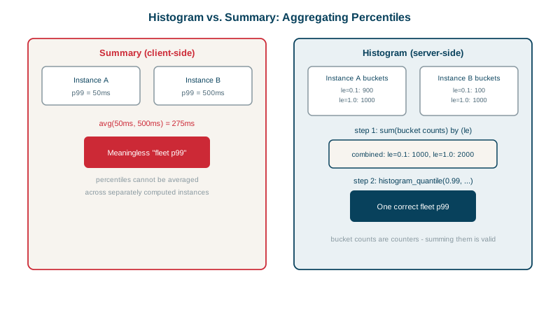
Each instance calculates its own p99 over a sliding window and exports it. Accurate per instance, but you can't combine them: there's no valid way to merge two p99 values into a p99 for the service.
Prometheus histograms: percentiles on the server
A histogram exports bucket counts (Day 5). Bucket counts can be summed across instances, and the percentile is calculated afterwards:
histogram_quantile(0.99,
  sum by (le) (rate(http_request_duration_seconds_bucket{route="/orders/:id/checkout"}[5m])))
Histogram vs summary accuracy: real numbers
Two instances, one slower than the other, with buckets [0.025, 0.05, 0.1, 0.25, 0.5, 1, 2.5]. Ground truth came from timing 3,000 requests directly in a client:
| Measure | Fast instance p99 | Slow instance p99 | Service p99 | Service p50 |
|---|---|---|---|---|
| Measured (truth) | 0.945 s | 1.235 s | 1.165 s | 0.206 s |
| Summary | 0.943 s | 1.173 s | n/a | n/a |
| Average of the two summary p99s | 1.058 s (meaningless) | |||
| Histogram | 0.726 s | 1.74 s | 0.996 s | 0.115 s |
What this shows:
- Summaries were accurate per instance, but the "service p99" from averaging them has no mathematical meaning. It happened to land near the truth here; with a different traffic split it can be wildly off.
- The histogram's service-level p99 is valid to compute, but its accuracy depends on buckets.
histogram_quantileassumes values are spread evenly within a bucket. The slow instance's true p99 (1.235 s) sits in the wide 1 to 2.5 s bucket, so it was estimated at 1.74 s. - The p50 was off by almost half: traffic is bimodal (fast instance around 46 ms, slow around 305 ms), and the median fell inside the 0.1 to 0.25 s bucket, where interpolation guessed wrong.
How to choose histogram buckets
- Put boundaries around your SLO thresholds: if the target is "99% under 300 ms", have a bucket at exactly 0.3. Then "fraction under 300 ms" is exact, even if percentile estimates aren't. In the lab, the fraction under 250 ms was a direct bucket ratio: 0.6045.
- More buckets where latency lives, fewer elsewhere. Each bucket adds a series per label combination (Day 7).
- Native histograms in recent Prometheus versions (and OpenTelemetry's exponential histograms) use automatically scaled buckets with much better precision at lower cost; prefer them where your stack supports them.
Histograms vs summaries: rules of thumb
- Use histograms for latency and sizes almost always.
- Use summaries only when you need precise per-instance quantiles and will never aggregate.
- Never average percentiles, whether from summaries or from per-instance histogram queries.
- Alert on "fraction of requests slower than X" (an SLO, Day 22) rather than on an interpolated p99.
Check yourself
Percentiles don't combine arithmetically. The service's p99 depends on the full latency distributions, and one slow instance with little traffic can skew an average of percentiles badly. Sum histogram buckets across instances first, then compute the quantile.
The true value fell in a wide bucket, from 1 to 2.5 seconds, and histogram_quantile assumes values are spread evenly within a bucket and interpolates linearly. Narrower buckets around the latencies you care about make estimates more accurate.
Place a boundary exactly at the SLO threshold, such as 300 ms, so the fraction of requests meeting it is measured exactly from bucket counts rather than estimated by interpolation. Error budget calculations then have no histogram error.
Each page view has 50 chances to hit a slow call; the chance that at least one is slower than p99 is about 1 - 0.99^50, roughly 40%.
Each instance computes its own quantiles, and quantiles can't be combined. Histograms keep bucket counts, which can be summed before computing a quantile.